A query takes 9 seconds. You read the SQL. You read EXPLAIN. Nothing looks wrong.
EXPLAIN tells you what ClickHouse® plans to do. It does not tell you where the 9 seconds actually went. For that you need to watch the query run - and that is what the CHOps Query Profiler does.
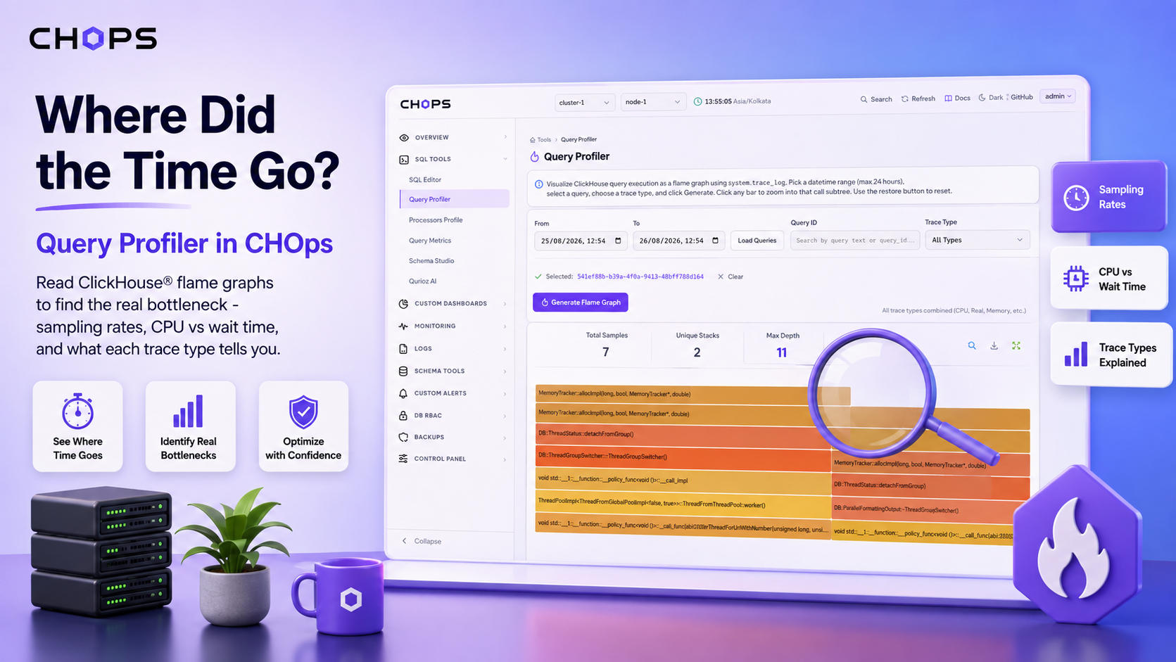
Open SQL Tools → Query Profiler, pick a query, and CHOps draws a flame graph of it.

What a flame graph actually is
A flame graph is a picture of where time went. That's it.
- The bottom bar is where the query starts.
- Every bar is one function that ran.
- Width = time. Wider bar, more time.
- Stacked bars = the call chain. A called B, B called C.
Read it bottom to top for what called what, left to right for what ran. But mostly you just find the widest bar. That's the bottleneck.
You do not need to know C++ or ClickHouse® internals for this. The function names carry enough meaning on their own:
| If the widest bar says… | The query is… |
|---|---|
ReadBufferFromFileDescriptor | IO-bound - reading too much from disk |
HashTable::insert | building hash tables for GROUP BY or JOIN |
MergeTreeDataSelectExecutor | scanning MergeTree parts - likely missing the primary index |
MemoryTracker::allocImpl | allocating - expected at the top of a memory trace |
Widest bar, read the name, act on it.
First, understand what a "sample" is
This is the part that trips people up, and it explains most of the confusion people have with the tool.
ClickHouse® does not record every function call. That would be ruinously slow. Instead it takes periodic snapshots: a timer fires, and whatever function each thread happens to be executing at that instant gets written as one row into system.trace_log. That row is one sample.
A flame graph is nothing more than those rows counted and stacked. Bar width = how many snapshots caught that function running.
By default ClickHouse® takes one snapshot per second, per thread:
| Sampling period | Snapshots/sec/thread | A 5s query on 4 threads gives |
|---|---|---|
1000000000 ns (1s - the default) | 1 | ~20 samples |
10000000 ns (10ms) | 100 | ~2,000 samples |
Twenty samples produce a few blocky bars and percentages that swing on every re-run. Two thousand produce a graph you can trust.
So if your flame graph looks thin, the query is usually fine - the sampling rate is the problem. Raise it for that one query:
SELECT ... your heavy query ...
SETTINGS
    query_profiler_real_time_period_ns = 10000000,
    query_profiler_cpu_time_period_ns  = 10000000;
Those go on the query you want to profile, when you run it. They change how ClickHouse® records that query while it executes. Nothing on the server changes, and no other query is affected.
Memory traces work on a different trigger: instead of a timer, ClickHouse® records a stack every time the query allocates another memory_profiler_step bytes (4 MiB by default). Lower that value for a denser memory graph.
The workflow
- Set From and To to when the query ran. The range is capped at 24 hours.
- Click Load Queries. The header shows how many queries in that window have trace data.
- Find your query. The picker searches by query text or query ID, and each row shows the ID, a SQL preview, the duration, the sample count and the timestamp.
- Click it - the selected ID appears below the list, with Clear beside it.
- Choose a Trace Type, then Generate Flame Graph.
The sample count in the list is the number to watch. Single digits means you're about to get a graph that tells you nothing; go back and re-run the query with a higher sampling rate.
Above the graph you get three quick stats: total samples, unique stacks, max depth. Unique stacks is the one people overlook - a low number means the query took very few distinct code paths, so there's little to see regardless of sample count.
If a query you just ran doesn't appear, run SYSTEM FLUSH LOGS;. Trace data is buffered before it's written.
Trace types: pick the one that matches your symptom
Nine options, and picking the right one matters more than anything else on the page.

| Trace Type | Answers | Use when |
|---|---|---|
| All Types | everything at once | first look, general orientation |
| CPU Time | where CPU went | the default choice for a slow query |
| Wall Clock (Real) | where clock time went, waits included | slow query, but CPU looks idle |
| Memory (Watermark) | what caused the biggest allocations | query was killed for memory |
| Memory (Sampled) | the spread of memory use | broad memory picture |
| Memory Peak | what was running at the memory high point | pinning down a spike |
| Profile Events | which internal counters moved most | advanced |
| Jemalloc Samples | what the allocator is doing | advanced - fragmentation debugging |
| Instrumentation | XRay instrumentation traces | advanced - needs SYSTEM INSTRUMENT |
Not all nine work out of the box. Some rely on collectors that are off by default, and if a collector is off you get an empty graph rather than an error. Worth knowing before you assume the tool is broken:
| Trace type | On a stock server |
|---|---|
| CPU Time, Wall Clock (Real) | work - but at 1 sample/sec/thread, thin |
| Memory (Watermark), Memory Peak | work - a stack every 4 MiB allocated |
| Memory (Sampled) | empty - needs memory_profiler_sample_probability > 0 |
| Profile Events | empty - needs trace_profile_events = 1 |
| Jemalloc Samples | empty unless the jemalloc profiler is enabled |
| Instrumentation | empty unless SYSTEM INSTRUMENT is on |
Check where you stand:
SELECT name, value
FROM system.settings
WHERE name LIKE '%profiler%' OR name = 'trace_profile_events';
The graph also re-labels itself for the trace type you picked. On a CPU or All Types graph the stats read total samples and the tooltip shows counts; switch to a memory type and the same line reads total bytes. A caption next to the Generate button spells out what the current selection measures.
Memory graphs get a second dropdown
Pick a memory trace type and a Memory Context filter appears next to it, with five options.

| Context | Shows |
|---|---|
| All Contexts | everything |
| Global (server) | server-wide allocations |
| User (user/merge) | user and merge allocations |
| Process (query) | just this query |
| Thread | thread-level allocations |
Choose Process (query) when debugging one query. Otherwise background merges and server caches get mixed into the graph and you end up optimising something unrelated.
Reading the shapes
One very wide bar. Easiest case. One function owns the query. Read its name, act on it.
Many narrow towers. Normal for queries with joins, subqueries and several aggregations - no single function dominates. Scan across all the towers for the widest single bar. Still your best lever.
Two towers of similar width. Work split across parallel paths. Widths are shares of the total, so two 50% towers means the cost is genuinely divided - fix both, or reduce the input feeding them.
Flat, no towers. One code path, or too few samples. Check the unique-stacks count before concluding anything about the query.
Hover any bar for its full function name and share of the total. Click to zoom into that subtree; the toolbox has restore, download and full-screen.

What CHOps is doing under the hood
No magic, and the UI doesn't hide it - a View Generated SQL panel under the graph shows the exact query CHOps ran:
SELECT
  arrayStringConcat(
    arrayReverse(arrayMap(x -> demangle(addressToSymbol(x)), trace)),
    ';'
  ) AS stack,
  count() AS samples
FROM system.trace_log
WHERE query_id = '...'
GROUP BY stack
SETTINGS allow_introspection_functions = 1addressToSymbolturns raw addresses into C++ symbolsdemanglemakes those symbols readablearrayReverseputs the root at the bottom, where a flame graph expects itGROUP BY stackcounts how often each call chain was sampled
CHOps folds those stacks into a tree and renders it. That folded-stack format is the same one every flame graph tool uses, which is why the output looks familiar if you've used perf.
Note this query only reads what was already captured. It can't create samples after the fact - which is why the sampling settings belong on the query you profile, not here.
Query Profiler or Processors Profile?
CHOps ships two profilers. Different tables, different questions.
| Query Profiler (flame graph) | Processors Profile (pipeline) | |
|---|---|---|
| Source | system.trace_log | system.processors_profile_log |
| Shows | C++ functions inside the engine | logical pipeline steps |
| Best for | engine-level debugging | day-to-day query optimisation |
| Example finding | most of the time in a read-pool function | ReadFromMergeTree 7.2s, AggregatingTransform 0.3s |
Start with Processors Profile. Its names map directly to query plan steps, so the fix is usually obvious. Switch to the Query Profiler when Processors Profile has told you which step is slow and you need to know why.
Before you get a graph
| Requirement | Why | Check |
|---|---|---|
system.trace_log enabled | that's where samples live | SELECT count() FROM system.trace_log |
allow_introspection_functions | needed for symbol resolution | CHOps passes it for you |
SELECT on system.trace_log, system.query_log | the CHOps ClickHouse® user needs read access | GRANT SELECT ON system.trace_log TO your_user |
clickhouse-common-static-dbg | optional - resolves system frames to names | dpkg -l clickhouse-common-static-dbg |
When it doesn't work
| Symptom | Cause | Fix |
|---|---|---|
| Graph is thin - a handful of bars | default 1 sample/sec/thread | re-run with query_profiler_*_period_ns = 10000000 |
| "No trace data found" | query finished before a snapshot fired | longer query, or a higher sampling rate |
| Empty graph on a specific trace type | that collector is off by default | see the trace-type table above |
| Query missing from the picker | trace data not flushed yet | SYSTEM FLUSH LOGS; |
| Bars show raw hex addresses | no debug symbols on the server | install clickhouse-common-static-dbg; only new traces resolve |
| Empty query list | nothing traced in that window | widen the range (up to 24h) |
Four habits worth forming
- Raise the sampling rate before you profile. More snapshots, better picture. This single setting is the difference between a useless graph and a useful one.
- Profile something heavy. A query finishing in milliseconds leaves almost nothing to sample, whatever the rate.
- Always compare CPU against Real. Fastest way to tell computation from waiting.
- Take a before and after. Generate a graph, add the index or projection, generate again. The change in bar widths is your proof the fix worked - a far better artifact for a PR than "feels faster now."
That last one is the real value. Flame graphs get sold as a diagnosis tool, but they're just as good as a verification tool. Optimisation without a before-and-after is guessing.
Try it
CHOps is free and open source.
- GitHub: https://github.com/Quantrail-Data/CH-Ops
- Docs: https://www.ch-ops.io/docs/guide/query-profiler
- Docker: https://hub.docker.com/r/quantrailadmin1/ch-ops
Run one slow query with the sampling rate turned up. Profile it. Look at the widest bar. You'll know more in thirty seconds than in an hour of reading EXPLAIN output.
Next in the CHOps series
Debugging Query Performance with Per-Second Metrics - Using CHOps