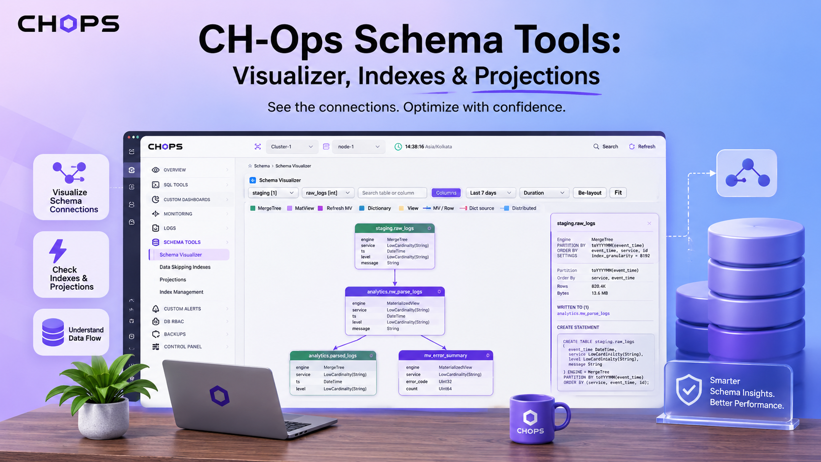
A ClickHouse® deployment rarely stays simple. A materialized view gets added to pre-aggregate something, then a second MV reads its output. A dictionary shows up for user lookups, a Distributed table sits in front of a sharded local table - and soon the schema is fully documented in DDL, and still hard to hold in your head.

The questions that come up are relational, not definitional:

• What feeds this table, and what does it feed?
• What breaks if I drop it?
• Which skipping indexes already exist here?
• Is there already a projection for this query pattern?
• How do I add or remove an index without hand-writing ALTER statements and remembering to backfill?

You can answer all of these by hand - SHOW CREATE TABLE, system.tables, cross-referencing MV definitions. It's just slow, and it gets worse fast once a pipeline crosses databases.

That's the gap Schema Tools in CH-Ops fills. Four screens - Schema Visualizer, Data Skipping Indexes, Projections, Index Management - read as one workflow: see how the schema connects, check what optimization already exists, weigh whether a projection helps, then manage indexes when the evidence supports it. It doesn't remove SQL - every index or projection action shows the exact statement before running it. What it removes is the friction around that: manual inspection, hand-written DDL, and the easy-to-miss materialization step.

The running example

Raw request logs land in staging.raw_logs. An MV parses them into analytics.parsed_logs - sorted by service, then time - which feeds two more MVs rolling requests into hourly metrics and error summaries, plus a Distributed table for sharded reads. A view in reporting aggregates the metrics for a dashboard. There's also analytics.users_dict, a dictionary loaded from a users table.

Keep that sort order - service, then time - in mind. It's what decides which queries are already fast.

Schema Visualizer: how is this schema connected?

Reconstructing a pipeline from DDL by hand means reading each MV's source and target and searching for anything downstream, one hop at a time. Cross-database dependencies are the worst case, since checking one database at a time hides them entirely.

The Schema Visualizer draws the graph instead: tables, MVs, dictionaries, Distributed tables, and views as cards, lines showing data flow. It's read-only - nothing here creates, alters, or drops anything.

It doesn't render the whole schema at once, on purpose - that's slow and unreadable. Pick a database, then a table, and CH-Ops traces every relationship in both directions, draws just that connected subgraph top to bottom, and auto-fits it.

The traversal isn't limited to one database. Starting at raw_logs pulls in all three databases on one canvas, each node labelled with its full name - the fastest way to find a dependency you didn't know existed.

Source at the top, transformations in the middle, destinations at the bottom - and three databases visible even though only one was selected.

Node types. Headers are colour-coded: MergeTree family (stores data), MaterializedView (fires on every insert), Refreshable MV (fires on a schedule), Dictionary, Distributed (routes to shards, stores nothing itself), View (a saved query, recomputed on read), Other. One glance tells you what stores data versus what just moves it.

Navigation. Dropdowns pick what's drawn. Search matches table and column names, highlighting hits and dimming the rest - handy for "which tables use user_id." Columns toggle switches between compact and detailed cards. Fit and Re-layout handle the camera and layout separately.

The sidebar. Click a node and it opens: engine, partition key, sort order, primary key (if different), rows/bytes, what it reads from, what reads from it, and the full CREATE statement. Reads/writes are clickable, so you can walk the pipeline hop by hop.

Capture parsed_logs selected - sort order and dependency list on one screen.

The heatmap. A graph shows how data moves, not what's doing the work. The optional heatmap covers that for MVs, over the last 1/7/30 days, built from system.query_views_log. On, it colours and thickens edges by view duration, rows/bytes written or read, peak memory, or executions - log-scaled, since volumes span orders of magnitude. Empty means no MVs fired, log_query_views is off, or the connecting user lacks SELECT on that table.

One hot edge next to cool ones makes the point: MVs at the same level of the graph don't cost the same to run.

Answers: how is my schema connected, and where does data flow?

Data Skipping Indexes: what already exists here?

An index doesn't sort anything - it summarizes each block (min/max, distinct values, a bloom filter, or text terms) so a filtering query can skip blocks that can't match. The sort key is what actually orders the data and makes those columns fast already. Indexes are for the filters the sort key doesn't cover.

On parsed_logs, service is already fast. user_id, status_code, and message are not.

The Data Skipping Indexes screen is read-only: database → table → each index, with type and covered expression, across everything.

The expression next to the type is the useful part - it catches a duplicate before you create it. Every index costs on every insert, so a duplicate is pure downside.

Four types:

• minmax - min/max per block. Cheap; great for dates and timestamps that correlate with insertion order.
• set - distinct values per block. Good for low-cardinality equality filters; useless past its size limit.
• bloom_filter - probabilistic; rules a block out for certain, but a "maybe" still means reading it. For equality on high-cardinality columns.
• text - indexes terms within a string, for searching rather than matching exactly.

Answers: what indexes does this table already have, and what are they indexing?

Projections: a different representation of the same data

A skipping index narrows a query. A projection changes what it reads from entirely - a second copy of the table, sorted differently or pre-aggregated. ClickHouse® decides on its own whether to use one; it's not free, and not an index.

Index → can I skip this block? Projection → is there a better-suited copy of this data?

Dashboards on this pipeline repeatedly ask for counts and latency by service and hour, recomputed every time. A pre-aggregated projection storing exactly that grouping solves it directly.

CH-Ops covers the lifecycle in five tabs: View (the same tree as the index screen), Add Projection (a form - table, name, select, optional grouping/ordering, cluster-wide and skip-if-exists options), Materialize Projection (builds it for existing rows), Clear Projection (empties data, keeps the definition), Drop Projection (removes it entirely). One quirk: projections don't support SELECT DISTINCT - CH-Ops strips it and tells you.

Capture two projections present, to show a table can carry more than one.

Grouping and ordering are separate fields - a projection grouped by day can't serve a query grouped by hour.

Creating isn't the same as filling.

Projection definition
        │
        ├── new inserts ──────────► maintained automatically
        │
        └── rows already in table ─► need Materialize Projection

New data is covered automatically; existing rows need materializing - real work on a big table, so it can be scoped per-partition to check whether it's worth it before doing the rest.

Capture the partition selector - controlled rebuild versus one long unbounded run.

Clear then rebuild is the fix for a drifted projection. Drop removes it for good. Either way, remember the cost: a projection is a second copy of the data, written on every insert whether it's used or not. Worth it for a query run constantly; not worth adding speculatively.

Answers: can I give ClickHouse® a better-suited representation for an important query pattern?

Index Management: create, materialize, drop

Three tabs - Create, Materialize, Drop - and this one needs admin access, unlike the read-only screens above.

Create. Database → table → column → name → type → granularity. The column list comes with data types attached, so there's no typing from memory. Some types add fields - bloom_filter a false-positive rate, text a tokenizer. Name it for what it does: idx_user_id, not idx1.

Granularity defaults to a sensible value and is one of the last things worth tuning - type and expression matter far more.

Materialize. Same gotcha as projections:

Create index  ──► applies to data inserted from now on
Materialize   ──► existing rows become covered

Nothing errors when this is skipped - the index just quietly doesn't help. Unlike projections, there's no partition-scoping option here - MATERIALIZE INDEX runs against the whole table in one go.

This screen is the answer to "I added the index and nothing changed."

Drop. Removes the index, not the data. Every index costs on writes for as long as it exists - if it's not earning that back, drop it. Normal tuning, not a mistake.

Answers: creating, materializing, and dropping - the three states of an index.

From schema discovery to optimization

1. Open the Visualizer, select parsed_logs.
2. See three MVs and a Distributed table depend on it.
3. Read the sort order from the sidebar.
4. Check Data Skipping Indexes for what's already covered.
5. Compare against your actual workload - endpoint/user filters aren't served by the sort key.
6. Check Projections for an existing pre-aggregation.
7. Decide: projection for a repeated aggregation, index for a plain filter.
8. Create it.
9. Materialize it.
10. Check whether it helped. Drop it if not.

CH-Ops doesn't tell you which index or projection to build - it shows what exists and where the load sits, then removes the DDL friction. The judgment calls (steps 5 and 7) are still yours, and the Query Profiler is where you confirm a query is actually slow before reaching for any of this.

Same table across all three panels - one object, four views of it.

Conclusion

Understand the schema, check what's already optimized, weigh a projection, manage indexes when the evidence supports it. The value isn't skipping SQL - you can write the DDL yourself, and CH-Ops shows you the statement anyway. It's having a fast, structured way to see what's already there before you touch it. Most bad schema decisions come from not seeing the dependency, the existing index, or the projection that was already there - not from an inability to write ALTER TABLE.

Pick your busiest table, open the Schema Visualizer, and see what's attached to it.

References

Schema Tools Documentation

Next in the CHOps series

Watch your clusters live on CHOps